Working with Conditional Formatting

Conditional formatting is a feature of Excel which allows you to apply a format to a cell or a range of cells based on certain criteria.

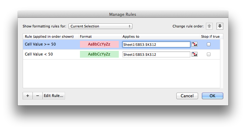
For example the following rules are used to highlight cells in the conditional_format.py example:

worksheet.conditional_format('B3:K12', {'type':     'cell',
                                        'criteria': '>=',
                                        'value':    50,
                                        'format':   format1})

worksheet.conditional_format('B3:K12', {'type':     'cell',
                                        'criteria': '<',
                                        'value':    50,
                                        'format':   format2})

Which gives criteria like this:

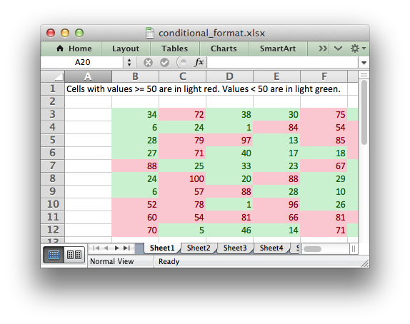
And output which looks like this:

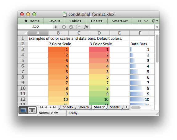
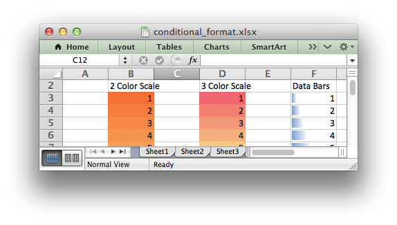
It is also possible to create color scales and data bars:

The conditional_format() method

The conditional_format() worksheet method is used to apply formatting based on user defined criteria to an XlsxWriter file.

The conditional format can be applied to a single cell or a range of cells. As usual you can use A1 or Row/Column notation (Working with Cell Notation).

With Row/Column notation you must specify all four cells in the range: (first_row, first_col, last_row, last_col). If you need to refer to a single cell set the last_* values equal to the first_* values. With A1 notation you can refer to a single cell or a range of cells:

worksheet.conditional_format(0, 0, 4, 1, {...})
worksheet.conditional_format('B1',       {...})
worksheet.conditional_format('C1:E5',    {...})

The options parameter in conditional_format() must be a dictionary containing the parameters that describe the type and style of the conditional format. The main parameters are:

type
format
criteria
value
minimum
maximum

Other, less commonly used parameters are:

min_type
mid_type
max_type
min_value
mid_value
max_value
min_color
mid_color
max_color
bar_color
bar_only
bar_solid
bar_negative_color
bar_border_color
bar_negative_border_color
bar_negative_color_same
bar_negative_border_color_same
bar_no_border
bar_direction
bar_axis_position
bar_axis_color
data_bar_2010
icon_style
icons
reverse_icons
icons_only
stop_if_true
multi_range

Conditional Format Options

The conditional format options that can be used with conditional_format() are explained in the following sections.

type

The type option is a required parameter and it has no default value. Allowable type values and their associated parameters are:

Type	Parameters
cell	criteria
	value
	minimum
	maximum
	format
date	criteria
	value
	minimum
	maximum
	format
time_period	criteria
	format
text	criteria
	value
	format
average	criteria
	format
duplicate	format
unique	format
top	criteria
	value
	format
bottom	criteria
	value
	format
blanks	format
no_blanks	format
errors	format
no_errors	format
formula	criteria
	format
2_color_scale	min_type
	max_type
	min_value
	max_value
	min_color
	max_color
3_color_scale	min_type
	mid_type
	max_type
	min_value
	mid_value
	max_value
	min_color
	mid_color
	max_color
data_bar	min_type
	max_type
	min_value
	max_value
	bar_only
	bar_color
	bar_solid*
	bar_negative_color*
	bar_border_color*
	bar_negative_border_color*
	bar_negative_color_same*
	bar_negative_border_color_same*
	bar_no_border*
	bar_direction*
	bar_axis_position*
	bar_axis_color*
	data_bar_2010*
icon_set	icon_style
	reverse_icons
	icons
	icons_only

Note

Data bar parameters marked with (*) are only available in Excel 2010 and later. Files that use these properties can still be opened in Excel 2007 but the data bars will be displayed without them.

type: cell

This is the most common conditional formatting type. It is used when a format is applied to a cell based on a simple criterion.

For example using a single cell and the greater than criteria:

worksheet.conditional_format('A1', {'type':     'cell',
                                    'criteria': 'greater than',
                                    'value':     5,
                                    'format':    red_format})

Or, using a range and the between criteria:

worksheet.conditional_format('C1:C4', {'type':     'cell',
                                       'criteria': 'between',
                                       'minimum':  20,
                                       'maximum':  30,
                                       'format':   green_format})

Other types are shown below, after the other main options.

criteria:

The criteria parameter is used to set the criteria by which the cell data will be evaluated. It has no default value. The most common criteria as applied to {'type': 'cell'} are:

`between`
`not between`
`equal to`	`==`
`not equal to`	`!=`
`greater than`	`>`
`less than`	`<`
`greater than or equal to`	`>=`
`less than or equal to`	`<=`

You can either use Excel’s textual description strings, in the first column above, or the more common symbolic alternatives.

Additional criteria which are specific to other conditional format types are shown in the relevant sections below.

value:

The value is generally used along with the criteria parameter to set the rule by which the cell data will be evaluated:

worksheet.conditional_format('A1', {'type':     'cell',
                                    'criteria': 'equal to',
                                    'value':    5,
                                    'format':   red_format})

If the type is cell and the value is a string then it should be double quoted, as required by Excel:

worksheet.conditional_format('A1', {'type':     'cell',
                                    'criteria': 'equal to',
                                    'value':    '"Failed"',
                                    'format':   red_format})

The value property can also be an cell reference:

worksheet.conditional_format('A1', {'type':     'cell',
                                    'criteria': 'equal to',
                                    'value':    '$C$1',
                                    'format':   red_format})

Note

In general any value property that refers to a cell reference should use an absolute reference, especially if the conditional formatting is applied to a range of values. Without an absolute cell reference the conditional format will not be applied correctly by Excel, apart from the first cell in the formatted range.

format:

The format parameter is used to specify the format that will be applied to the cell when the conditional formatting criterion is met. The format is created using the add_format() method in the same way as cell formats:

format1 = workbook.add_format({'bold': 1, 'italic': 1})

worksheet.conditional_format('A1', {'type':     'cell',
                                    'criteria': '>',
                                    'value':    5,
                                    'format':   format1})

Note

In Excel, a conditional format is superimposed over the existing cell format and not all cell format properties can be modified. Properties that cannot be modified in a conditional format are font name, font size, superscript and subscript, diagonal borders, all alignment properties and all protection properties.

Excel specifies some default formats to be used with conditional formatting. These can be replicated using the following XlsxWriter formats:

# Light red fill with dark red text.
format1 = workbook.add_format({'bg_color':   '#FFC7CE',
                               'font_color': '#9C0006'})

# Light yellow fill with dark yellow text.
format2 = workbook.add_format({'bg_color':   '#FFEB9C',
                               'font_color': '#9C6500'})

# Green fill with dark green text.
format3 = workbook.add_format({'bg_color':   '#C6EFCE',
                               'font_color': '#006100'})

minimum:

The minimum parameter is used to set the lower limiting value when the criteria is either 'between' or 'not between':

worksheet.conditional_format('A1', {'type':     'cell',
                                    'criteria': 'between',
                                    'minimum':  2,
                                    'maximum':  6,
                                    'format':   format1,
                                    })

maximum:

The maximum parameter is used to set the upper limiting value when the criteria is either 'between' or 'not between'. See the previous example.

type: date

The date type is similar the cell type and uses the same criteria and values. However, the value, minimum and maximum properties are specified as a datetime object as shown in Working with Dates and Time:

date = datetime.datetime.strptime('2011-01-01', "%Y-%m-%d")

worksheet.conditional_format('A1:A4', {'type':     'date',
                                       'criteria': 'greater than',
                                       'value':    date,
                                       'format':   format1})

type: time_period

The time_period type is used to specify Excel’s “Dates Occurring” style conditional format:

worksheet.conditional_format('A1:A4', {'type':     'time_period',
                                       'criteria': 'yesterday',
                                       'format':   format1})

The period is set in the criteria and can have one of the following values:

'criteria': 'yesterday',
'criteria': 'today',
'criteria': 'last 7 days',
'criteria': 'last week',
'criteria': 'this week',
'criteria': 'next week',
'criteria': 'last month',
'criteria': 'this month',
'criteria': 'next month'

type: text

The text type is used to specify Excel’s “Specific Text” style conditional format. It is used to do simple string matching using the criteria and value parameters:

worksheet.conditional_format('A1:A4', {'type':     'text',
                                       'criteria': 'containing',
                                       'value':    'foo',
                                       'format':   format1})

The criteria can have one of the following values:

'criteria': 'containing',
'criteria': 'not containing',
'criteria': 'begins with',
'criteria': 'ends with',

The value parameter should be a string or single character.

type: average

The average type is used to specify Excel’s “Average” style conditional format:

worksheet.conditional_format('A1:A4', {'type':     'average',
                                       'criteria': 'above',
                                       'format':   format1})

The type of average for the conditional format range is specified by the criteria:

'criteria': 'above',
'criteria': 'below',
'criteria': 'equal or above',
'criteria': 'equal or below',
'criteria': '1 std dev above',
'criteria': '1 std dev below',
'criteria': '2 std dev above',
'criteria': '2 std dev below',
'criteria': '3 std dev above',
'criteria': '3 std dev below',

type: duplicate

The duplicate type is used to highlight duplicate cells in a range:

worksheet.conditional_format('A1:A4', {'type':   'duplicate',
                                       'format': format1})

type: unique

The unique type is used to highlight unique cells in a range:

worksheet.conditional_format('A1:A4', {'type':   'unique',
                                       'format': format1})

type: top

The top type is used to specify the top n values by number or percentage in a range:

worksheet.conditional_format('A1:A4', {'type':   'top',
                                       'value':  10,
                                       'format': format1})

The criteria can be used to indicate that a percentage condition is required:

worksheet.conditional_format('A1:A4', {'type':     'top',
                                       'value':    10,
                                       'criteria': '%',
                                       'format':   format1})

type: bottom

The bottom type is used to specify the bottom n values by number or percentage in a range.

It takes the same parameters as top, see above.

type: blanks

The blanks type is used to highlight blank cells in a range:

worksheet.conditional_format('A1:A4', {'type':   'blanks',
                                       'format': format1})

type: no_blanks

The no_blanks type is used to highlight non blank cells in a range:

worksheet.conditional_format('A1:A4', {'type':   'no_blanks',
                                       'format': format1})

type: errors

The errors type is used to highlight error cells in a range:

worksheet.conditional_format('A1:A4', {'type':   'errors',
                                       'format': format1})

type: no_errors

The no_errors type is used to highlight non error cells in a range:

worksheet.conditional_format('A1:A4', {'type':   'no_errors',
                                       'format': format1})

type: formula

The formula type is used to specify a conditional format based on a user defined formula:

worksheet.conditional_format('A1:A4', {'type':     'formula',
                                       'criteria': '=$A$1>5',
                                       'format':   format1})

The formula is specified in the criteria.

Formulas must be written with the US style separator/range operator which is a comma (not semi-colon) and should follow the same rules as write_formula(). See Non US Excel functions and syntax for a full explanation:

# This formula will cause an Excel error on load due to
# non-English language and use of semi-colons.
worksheet.conditional_format('A2:C9' ,
    {'type':     'formula',
     'criteria': '=ODER($B2<$C2;UND($B2="";$C2>HEUTE()))',
     'format':   format1
    })

# This is the correct syntax.
worksheet.conditional_format('A2:C9' ,
    {'type':     'formula',
     'criteria': '=OR($B2<$C2,AND($B2="",$C2>TODAY()))',
     'format':   format1
    })

Also, any cell or range references in the formula should be absolute references if they are applied to the full range of the conditional format. See the note in the value section above.

type: 2_color_scale

The 2_color_scale type is used to specify Excel’s “2 Color Scale” style conditional format:

worksheet.conditional_format('A1:A12', {'type': '2_color_scale'})

This conditional type can be modified with min_type, max_type, min_value, max_value, min_color and max_color, see below.

type: 3_color_scale

The 3_color_scale type is used to specify Excel’s “3 Color Scale” style conditional format:

worksheet.conditional_format('A1:A12', {'type': '3_color_scale'})

This conditional type can be modified with min_type, mid_type, max_type, min_value, mid_value, max_value, min_color, mid_color and max_color, see below.

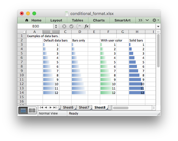
type: data_bar

The data_bar type is used to specify Excel’s “Data Bar” style conditional format:

worksheet.conditional_format('A1:A12', {'type': 'data_bar'})

This conditional type can be modified with the following parameters, which are explained in the sections below. These properties were available in the original xlsx file specification used in Excel 2007:

min_type
max_type
min_value
max_value
bar_color
bar_only

In Excel 2010 additional data bar properties were added such as solid (non-gradient) bars and control over how negative values are displayed. These properties can be set using the following parameters:

bar_solid
bar_negative_color
bar_border_color
bar_negative_border_color
bar_negative_color_same
bar_negative_border_color_same
bar_no_border
bar_direction
bar_axis_position
bar_axis_color
data_bar_2010

Files that use these Excel 2010 properties can still be opened in Excel 2007 but the data bars will be displayed without them.

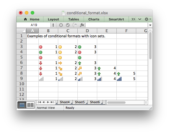
type: icon_set

The icon_set type is used to specify a conditional format with a set of icons such as traffic lights or arrows:

worksheet.conditional_format('A1:C1', {'type': 'icon_set',
                                       'icon_style': '3_traffic_lights'})

The icon set style is specified by the icon_style parameter. Valid options are:

3_arrows
3_arrows_gray
3_flags
3_signs
3_symbols
3_symbols_circled
3_traffic_lights
3_traffic_lights_rimmed

4_arrows
4_arrows_gray
4_ratings
4_red_to_black
4_traffic_lights

5_arrows
5_arrows_gray
5_quarters
5_ratings

The criteria, type and value of each icon can be specified using the icon array of dicts with optional criteria, type and value parameters:

worksheet.conditional_format(
    'A1:D1',
    {'type': 'icon_set',
     'icon_style': '4_red_to_black',
     'icons': [{'criteria': '>=', 'type': 'number',     'value': 90},
               {'criteria': '<',  'type': 'percentile', 'value': 50},
               {'criteria': '<=', 'type': 'percent',    'value': 25}]}
)

The icons criteria parameter should be either >= or <. The default criteria is >=.
The icons type parameter should be one of the following values:
```
number
percentile
percent
formula
```
The default type is percent.

The icons value parameter can be a value or formula:

worksheet.conditional_format('A1:D1',
                             {'type': 'icon_set',
                              'icon_style': '4_red_to_black',
                              'icons': [{'value': 90},
                                        {'value': 50},
                                        {'value': 25}]})

Note: The icons parameters should start with the highest value and with each subsequent one being lower. The default value is (n * 100) / number_of_icons. The lowest number icon in an icon set has properties defined by Excel. Therefore in a n icon set, there is no n-1 hash of parameters.

The order of the icons can be reversed using the reverse_icons parameter:

worksheet.conditional_format('A1:C1',
                             {'type': 'icon_set',
                              'icon_style': '3_arrows',
                              'reverse_icons': True})

The icons can be displayed without the cell value using the icons_only parameter:

worksheet.conditional_format('A1:C1',
                             {'type': 'icon_set',
                              'icon_style': '3_flags',
                              'icons_only': True})

min_type:

The min_type and max_type properties are available when the conditional formatting type is 2_color_scale, 3_color_scale or data_bar. The mid_type is available for 3_color_scale. The properties are used as follows:

worksheet.conditional_format('A1:A12', {'type':     '2_color_scale',
                                        'min_type': 'percent',
                                        'max_type': 'percent'})

The available min/mid/max types are:

min        (for min_type only)
num
percent
percentile
formula
max        (for max_type only)

mid_type:

Used for 3_color_scale. Same as min_type, see above.

max_type:

Same as min_type, see above.

min_value:

The min_value and max_value properties are available when the conditional formatting type is 2_color_scale, 3_color_scale or data_bar. The mid_value is available for 3_color_scale. The properties are used as follows:

worksheet.conditional_format('A1:A12', {'type':      '2_color_scale',
                                        'min_value': 10,
                                        'max_value': 90})

mid_value:

Used for 3_color_scale. Same as min_value, see above.

max_value:

Same as min_value, see above.

min_color:

The min_color and max_color properties are available when the conditional formatting type is 2_color_scale, 3_color_scale or data_bar. The mid_color is available for 3_color_scale. The properties are used as follows:

worksheet.conditional_format('A1:A12', {'type':      '2_color_scale',
                                        'min_color': '#C5D9F1',
                                        'max_color': '#538ED5'})

The color can be a Html style #RRGGBB string or a limited number named colors, see Working with Colors.

mid_color:

Used for 3_color_scale. Same as min_color, see above.

max_color:

Same as min_color, see above.

bar_color:

The bar_color parameter sets the fill color for data bars:

worksheet.conditional_format('F3:F14', {'type': 'data_bar',
                                        'bar_color': '#63C384'})

The color can be a Html style #RRGGBB string or a limited number named colors, see Working with Colors.

bar_only:

The bar_only property displays a bar data but not the data in the cells:

worksheet.conditional_format('D3:D14', {'type': 'data_bar',
                                        'bar_only': True})

See the image above.

bar_solid:

The bar_solid property turns on a solid (non-gradient) fill for data bars:

worksheet.conditional_format('H3:H14', {'type': 'data_bar',
                                        'bar_solid': True})

See the image above.

Note, this property is only visible in Excel 2010 and later.

bar_negative_color:

The bar_negative_color property sets the color fill for the negative portion of a data bar:

worksheet.conditional_format('F3:F14', {'type': 'data_bar',
                                        'bar_negative_color': '#63C384'})

The color can be a Html style #RRGGBB string or a limited number named colors, see Working with Colors.

Note, this property is only visible in Excel 2010 and later.

bar_border_color:

The bar_border_color property sets the color for the border line of a data bar:

worksheet.conditional_format('F3:F14', {'type': 'data_bar',
                                        'bar_border_color': '#63C384'})

The color can be a Html style #RRGGBB string or a limited number named colors, see Working with Colors.

Note, this property is only visible in Excel 2010 and later.

bar_negative_border_color:

The bar_negative_border_color property sets the color for the border of the negative portion of a data bar:

worksheet.conditional_format('F3:F14', {'type': 'data_bar',
                                        'bar_negative_border_color': '#63C384'})

The color can be a Html style #RRGGBB string or a limited number named colors, see Working with Colors.

Note, this property is only visible in Excel 2010 and later.

bar_negative_color_same:

The bar_negative_color_same property sets the fill color for the negative portion of a data bar to be the same as the fill color for the positive portion of the data bar:

worksheet.conditional_format('F3:F14', {'type': 'data_bar',
                                        'bar_negative_color_same': True})

Note, this property is only visible in Excel 2010 and later.

bar_negative_border_color_same:

The bar_negative_border_color_same property sets the border color for the negative portion of a data bar to be the same as the border color for the positive portion of the data bar:

worksheet.conditional_format('F3:F14', {'type': 'data_bar',
                                        'bar_negative_border_color_same': True})

See the image above.

Note, this property is only visible in Excel 2010 and later.

bar_no_border:

The bar_no_border property turns off the border for data bars:

worksheet.conditional_format('F3:F14', {'type': 'data_bar',
                                        'bar_no_border': True})

Note, this property is only visible in Excel 2010 and later, however the default in Excel 2007 is to not have a border.

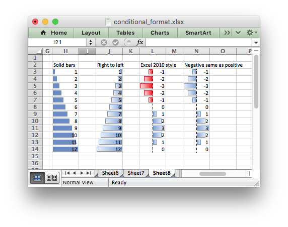
bar_direction:

The bar_direction property sets the direction for data bars. This property can be either left for left-to-right or right for right-to-left. If the property isn’t set then Excel will adjust the position automatically based on the context:

worksheet.conditional_format('J3:J14', {'type': 'data_bar',
                                        'bar_direction': 'right'})

Note, this property is only visible in Excel 2010 and later.

bar_axis_position:

The bar_axis_position property sets the position within the cells for the axis that is shown in data bars when there are negative values to display. The property can be either middle or none. If the property isn’t set then Excel will position the axis based on the range of positive and negative values:

worksheet.conditional_format('J3:J14', {'type': 'data_bar',
                                        'bar_axis_position': 'middle'})

Note, this property is only visible in Excel 2010 and later.

bar_axis_color:

The bar_axis_color property sets the color for the axis that is shown in data bars when there are negative values to display:

worksheet.conditional_format('J3:J14', {'type': 'data_bar',
                                        'bar_axis_color': '#0070C0'})

Note, this property is only visible in Excel 2010 and later.

data_bar_2010:

The data_bar_2010 property sets Excel 2010 style data bars even when Excel 2010 specific properties aren’t used. This can be used for consistency across all the data bar formatting in a worksheet:

worksheet.conditional_format('L3:L14', {'type': 'data_bar',
                                        'data_bar_2010': True})

stop_if_true

The stop_if_true parameter can be used to set the “stop if true” feature of a conditional formatting rule when more than one rule is applied to a cell or a range of cells. When this parameter is set then subsequent rules are not evaluated if the current rule is true:

worksheet.conditional_format('A1',
                             {'type': 'cell',
                              'format': cell_format,
                              'criteria': '>',
                              'value': 20,
                              'stop_if_true': True
                              })

multi_range:

The multi_range option is used to extend a conditional format over non-contiguous ranges.

It is possible to apply the conditional format to different cell ranges in a worksheet using multiple calls to conditional_format(). However, as a minor optimization it is also possible in Excel to apply the same conditional format to different non-contiguous cell ranges.

This is replicated in conditional_format() using the multi_range option. The range must contain the primary range for the conditional format and any others separated by spaces.

For example to apply one conditional format to two ranges, 'B3:K6' and 'B9:K12':

worksheet.conditional_format('B3:K6', {'type': 'cell',
                                       'criteria': '>=',
                                       'value': 50,
                                       'format': format1,
                                       'multi_range': 'B3:K6 B9:K12'})

Conditional Formatting Examples

Highlight cells greater than an integer value:

worksheet.conditional_format('A1:F10', {'type':     'cell',
                                        'criteria': 'greater than',
                                        'value':    5,
                                        'format':   format1})

Highlight cells greater than a value in a reference cell:

worksheet.conditional_format('A1:F10', {'type':     'cell',
                                        'criteria': 'greater than',
                                        'value':    'H1',
                                        'format':   format1})

Highlight cells more recent (greater) than a certain date:

date = datetime.datetime.strptime('2011-01-01', "%Y-%m-%d")

worksheet.conditional_format('A1:F10', {'type':     'date',
                                        'criteria': 'greater than',
                                        'value':    date,
                                        'format':   format1})

Highlight cells with a date in the last seven days:

worksheet.conditional_format('A1:F10', {'type':     'time_period',
                                        'criteria': 'last 7 days',
                                        'format':   format1})

Highlight cells with strings starting with the letter b:

worksheet.conditional_format('A1:F10', {'type':     'text',
                                        'criteria': 'begins with',
                                        'value':    'b',
                                        'format':   format1})

Highlight cells that are 1 standard deviation above the average for the range:

worksheet.conditional_format('A1:F10', {'type':   'average',
                                        'format': format1})

Highlight duplicate cells in a range:

worksheet.conditional_format('A1:F10', {'type':   'duplicate',
                                        'format': format1})

Highlight unique cells in a range:

worksheet.conditional_format('A1:F10', {'type':   'unique',
                                        'format': format1})

Highlight the top 10 cells:

worksheet.conditional_format('A1:F10', {'type':   'top',
                                        'value':  10,
                                        'format': format1})

Highlight blank cells:

worksheet.conditional_format('A1:F10', {'type':   'blanks',
                                        'format': format1})

Set traffic light icons in 3 cells:

worksheet.conditional_format('B3:D3', {'type': 'icon_set',
                                       'icon_style': '3_traffic_lights'})