Working with Formulas

In general a formula in Excel can be used directly in the write_formula() method:

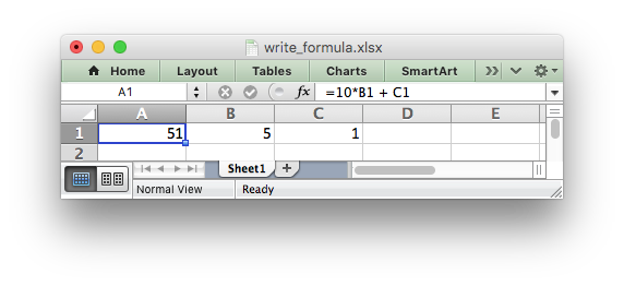
worksheet.write_formula('A1', '=10*B1 + C1')

However, there are a few potential issues and differences that the user should be aware of. These are explained in the following sections.

Non US Excel functions and syntax

Excel stores formulas in the format of the US English version, regardless of the language or locale of the end-user’s version of Excel. Therefore all formula function names written using XlsxWriter must be in English:

worksheet.write_formula('A1', '=SUM(1, 2, 3)')    # OK
worksheet.write_formula('A2', '=SOMME(1, 2, 3)')  # French. Error on load.

Also, formulas must be written with the US style separator/range operator which is a comma (not semi-colon). Therefore a formula with multiple values should be written as follows:

worksheet.write_formula('A1', '=SUM(1, 2, 3)')   # OK
worksheet.write_formula('A2', '=SUM(1; 2; 3)')   # Semi-colon. Error on load.

If you have a non-English version of Excel you can use the following multi-lingual formula translator to help you convert the formula. It can also replace semi-colons with commas.

Formula Results

XlsxWriter doesn’t calculate the result of a formula and instead stores the value 0 as the formula result. It then sets a global flag in the XLSX file to say that all formulas and functions should be recalculated when the file is opened.

This is the method recommended in the Excel documentation and in general it works fine with spreadsheet applications. However, applications that don’t have a facility to calculate formulas will only display the 0 results. Examples of such applications are Excel Viewer, PDF Converters, and some mobile device applications.

If required, it is also possible to specify the calculated result of the formula using the optional value parameter for write_formula():

worksheet.write_formula('A1', '=2+2', num_format, 4)

The value parameter can be a number, a string, a bool or one of the following Excel error codes:

#DIV/0!
#N/A
#NAME?
#NULL!
#NUM!
#REF!
#VALUE!

It is also possible to specify the calculated result of an array formula created with write_array_formula():

# Specify the result for a single cell range.
worksheet.write_array_formula('A1:A1', '{=SUM(B1:C1*B2:C2)}', cell_format, 2005)

However, using this parameter only writes a single value to the upper left cell in the result array. For a multi-cell array formula where the results are required, the other result values can be specified by using write_number() to write to the appropriate cell:

# Specify the results for a multi cell range.
worksheet.write_array_formula('A1:A3', '{=TREND(C1:C3,B1:B3)}', cell_format, 15)
worksheet.write_number('A2', 12, cell_format)
worksheet.write_number('A3', 14, cell_format)

Dynamic Array support

Excel introduced the concept of “Dynamic Arrays” and new functions that use them in Office 365. The new functions are:

BYCOL()
BYROW()
CHOOSECOLS()
CHOOSEROWS()
DROP()
EXPAND()
FILTER()
HSTACK()
MAKEARRAY()
MAP()
RANDARRAY()
REDUCE()
SCAN()
SEQUENCE()
SORT()
SORTBY()
SWITCH()
TAKE()
TEXTSPLIT()
TOCOL()
TOROW()
UNIQUE()
VSTACK()
WRAPCOLS()
WRAPROWS()
XLOOKUP()

The following special case functions were also added with Dynamic Arrays:

SINGLE() - Explained below in Dynamic Arrays - The Implicit Intersection Operator “@”.
ANCHORARRAY() - Explained below in Dynamic Arrays - The Spilled Range Operator “#”.
LAMBDA() and LET() - Explained below in The Excel 365 LAMBDA() function.

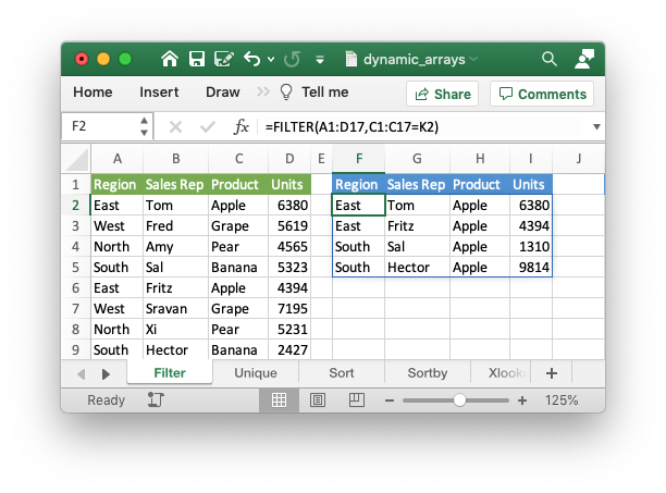
Dynamic arrays are ranges of return values that can change in size based on the results. For example, a function such as FILTER() returns an array of values that can vary in size depending on the filter results. This is shown in the snippet below from Example: Dynamic array formulas:

worksheet1.write('F2', '=FILTER(A1:D17,C1:C17=K2)')

Which gives the results shown in the image below. The dynamic range here is “F2:I5” but it could be different based on the filter criteria.

It is also possible to get dynamic array behavior with older Excel functions. For example, the Excel function =LEN(A1) applies to a single cell and returns a single value but it is also possible to apply it to a range of cells and return a range of values using an array formula like {=LEN(A1:A3)}. This type of “static” array behavior is called a CSE (Ctrl+Shift+Enter) formula. With the introduction of dynamic arrays in Excel 365 you can now write this function as =LEN(A1:A3) and get a dynamic range of return values. 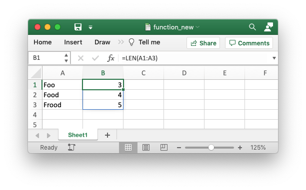In XlsxWriter you can use the write_array_formula() worksheet method to get a static/CSE range and write_dynamic_array_formula() to get a dynamic range. For example:

worksheet.write_dynamic_array_formula('B1:B3', '=LEN(A1:A3)')

Which gives the following result:

The difference between the two types of array functions is explained in the Microsoft documentation on Dynamic array formulas vs. legacy CSE array formulas. Note the use of the word “legacy” here. This, and the documentation itself, is a clear indication of the future importance of dynamic arrays in Excel.

For a wider and more general introduction to dynamic arrays see the following: Dynamic array formulas in Excel.

Dynamic Arrays - The Implicit Intersection Operator “@”

The Implicit Intersection Operator, “@”, is used by Excel 365 to indicate a position in a formula that is implicitly returning a single value when a range or an array could be returned.

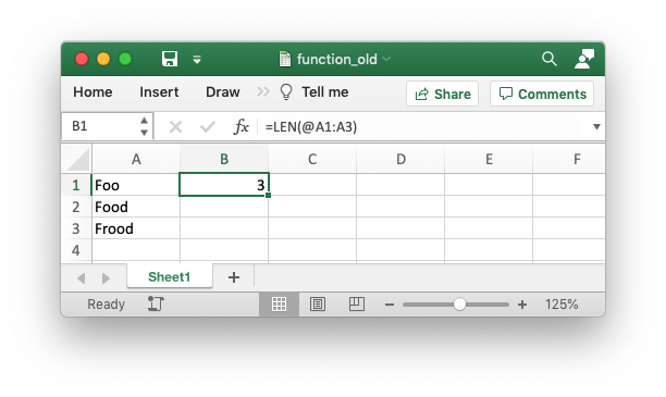
We can see how this operator works in practice by considering the formula we used in the last section: =LEN(A1:A3). In Excel versions without support for dynamic arrays, i.e. prior to Excel 365, this formula would operate on a single value from the input range and return a single value, like this:

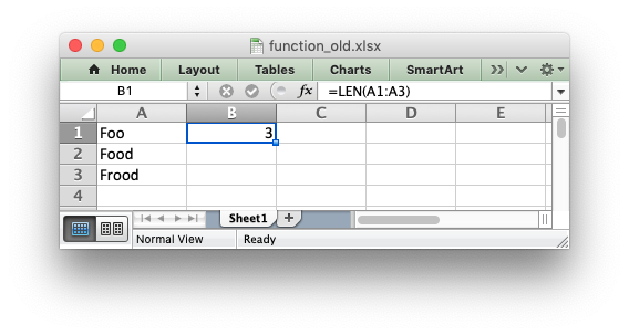
There is an implicit conversion here of the range of input values, “A1:A3”, to a single value “A1”. Since this was the default behavior of older versions of Excel this conversion isn’t highlighted in any way. But if you open the same file in Excel 365 it will appear as follows:

The result of the formula is the same (this is important to note) and it still operates on, and returns, a single value. However the formula now contains a “@” operator to show that it is implicitly using a single value from the given range.

Finally, if you entered this formula in Excel 365, or with write_dynamic_array_formula() in XlsxWriter, it would operate on the entire range and return an array of values:

If you are encountering the Implicit Intersection Operator “@” for the first time then it is probably from a point of view of “why is Excel/XlsxWriter putting @s in my formulas”. In practical terms if you encounter this operator, and you don’t intend it to be there, then you should probably write the formula as a CSE or dynamic array function using write_array_formula() or write_dynamic_array_formula() (see the previous section on Dynamic Array support).

A full explanation of this operator is shown in the Microsoft documentation on the Implicit intersection operator: @.

One important thing to note is that the “@” operator isn’t stored with the formula. It is just displayed by Excel 365 when reading “legacy” formulas. However, it is possible to write it to a formula, if necessary, using SINGLE() or _xlfn.SINGLE(). The unusual cases where this may be necessary are shown in the linked document in the previous paragraph.

Dynamic Arrays - The Spilled Range Operator “#”

In the section above on Dynamic Array support we saw that dynamic array formulas can return variable sized ranges of results. The Excel documentation refers to this as a “Spilled” range/array from the idea that the results spill into the required number of cells. This is explained in the Microsoft documentation on Dynamic array formulas and spilled array behavior.

Since a spilled range is variable in size a new operator is required to refer to the range. This operator is the Spilled range operator and it is represented by “#”. For example, the range F2# in the image below is used to refer to a dynamic array returned by UNIQUE() in the cell F2. This example is taken from the XlsxWriter program Example: Dynamic array formulas.

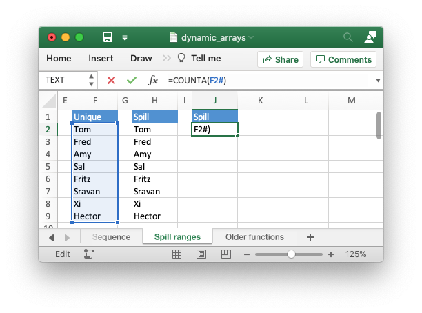
Unfortunately, Excel doesn’t store the formula like this and in XlsxWriter you need to use the explicit function ANCHORARRAY() to refer to a spilled range. The example in the image above was generated using the following:

worksheet9.write('J2', '=COUNTA(ANCHORARRAY(F2))')  # Same as '=COUNTA(F2#)' in Excel.

The Excel 365 LAMBDA() function

Recent versions of Excel 365 have introduced a powerful new function/feature called LAMBDA(). This is similar to the lambda function in Python (and other languages).

Consider the following Excel example which converts the variable temp from Fahrenheit to Celsius:

LAMBDA(temp, (5/9) * (temp-32))

This could be called in Excel with an argument:

=LAMBDA(temp, (5/9) * (temp-32))(212)

Or assigned to a defined name and called as a user defined function:

=ToCelsius(212)

This is similar to this example in Python:

>>> to_celsius = lambda temp: (5.0/9.0) * (temp-32)
>>> to_celsius(212)
100.0

A XlsxWriter program that replicates the Excel is shown in Example: Excel 365 LAMBDA() function.

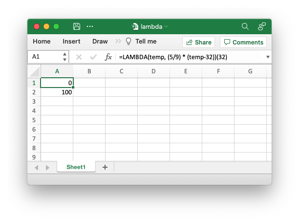
The formula is written as follows:

worksheet.write('A2', '=LAMBDA(_xlpm.temp, (5/9) * (_xlpm.temp-32))(32)')

Note, that the parameters in the LAMBDA() function must have a “_xlpm.” prefix for compatibility with how the formulas are stored in Excel. These prefixes won’t show up in the formula, as shown in the image.

The LET() function is often used in conjunction with LAMBDA() to assign names to calculation results.

Formulas added in Excel 2010 and later

Excel 2010 and later added functions which weren’t defined in the original file specification. These functions are referred to by Microsoft as future functions. Examples of these functions are ACOT, CHISQ.DIST.RT , CONFIDENCE.NORM, STDEV.P, STDEV.S and WORKDAY.INTL.

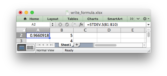
When written using write_formula() these functions need to be fully qualified with a _xlfn. (or other) prefix as they are shown the list below. For example:

worksheet.write_formula('A1', '=_xlfn.STDEV.S(B1:B10)')

These functions will appear without the prefix in Excel:

Alternatively, you can enable the use_future_functions option in the Workbook() constructor, which will add the prefix as required:

workbook = Workbook('write_formula.xlsx', {'use_future_functions': True})

# ...

worksheet.write_formula('A1', '=STDEV.S(B1:B10)')

If the formula already contains a _xlfn. prefix, on any function, then the formula will be ignored and won’t be expanded any further.

Note

Enabling the use_future_functions option adds an overhead to all formula processing in XlsxWriter. If your application has a lot of formulas or is performance sensitive then it is best to use the explicit _xlfn. prefix instead.

The following list is taken from MS XLSX extensions documentation on future functions.

_xlfn.ACOTH
_xlfn.ACOT
_xlfn.AGGREGATE
_xlfn.ARABIC
_xlfn.ARRAYTOTEXT
_xlfn.BASE
_xlfn.BETA.DIST
_xlfn.BETA.INV
_xlfn.BINOM.DIST.RANGE
_xlfn.BINOM.DIST
_xlfn.BINOM.INV
_xlfn.BITAND
_xlfn.BITLSHIFT
_xlfn.BITOR
_xlfn.BITRSHIFT
_xlfn.BITXOR
_xlfn.CEILING.MATH
_xlfn.CEILING.PRECISE
_xlfn.CHISQ.DIST.RT
_xlfn.CHISQ.DIST
_xlfn.CHISQ.INV.RT
_xlfn.CHISQ.INV
_xlfn.CHISQ.TEST
_xlfn.COMBINA
_xlfn.CONCAT
_xlfn.CONFIDENCE.NORM
_xlfn.CONFIDENCE.T
_xlfn.COTH
_xlfn.COT
_xlfn.COVARIANCE.P
_xlfn.COVARIANCE.S
_xlfn.CSCH
_xlfn.CSC
_xlfn.DAYS
_xlfn.DECIMAL
ECMA.CEILING
_xlfn.ERF.PRECISE
_xlfn.ERFC.PRECISE
_xlfn.EXPON.DIST
_xlfn.F.DIST.RT
_xlfn.F.DIST
_xlfn.F.INV.RT
_xlfn.F.INV
_xlfn.F.TEST
_xlfn.FILTERXML
_xlfn.FLOOR.MATH
_xlfn.FLOOR.PRECISE
_xlfn.FORECAST.ETS.CONFINT
_xlfn.FORECAST.ETS.SEASONALITY
_xlfn.FORECAST.ETS.STAT
_xlfn.FORECAST.ETS
_xlfn.FORECAST.LINEAR
_xlfn.FORMULATEXT
_xlfn.GAMMA.DIST
_xlfn.GAMMA.INV
_xlfn.GAMMALN.PRECISE
_xlfn.GAMMA
_xlfn.GAUSS
_xlfn.HYPGEOM.DIST
_xlfn.IFNA
_xlfn.IFS
_xlfn.IMAGE
_xlfn.IMCOSH
_xlfn.IMCOT
_xlfn.IMCSCH
_xlfn.IMCSC
_xlfn.IMSECH
_xlfn.IMSEC
_xlfn.IMSINH
_xlfn.IMTAN
_xlfn.ISFORMULA
_xlfn.ISOMITTED
_xlfn.ISOWEEKNUM
_xlfn.LET
_xlfn.LOGNORM.DIST
_xlfn.LOGNORM.INV
_xlfn.MAXIFS
_xlfn.MINIFS
_xlfn.MODE.MULT
_xlfn.MODE.SNGL
_xlfn.MUNIT
_xlfn.NEGBINOM.DIST
NETWORKDAYS.INTL
_xlfn.NORM.DIST
_xlfn.NORM.INV
_xlfn.NORM.S.DIST
_xlfn.NORM.S.INV
_xlfn.NUMBERVALUE
_xlfn.PDURATION
_xlfn.PERCENTILE.EXC
_xlfn.PERCENTILE.INC
_xlfn.PERCENTRANK.EXC
_xlfn.PERCENTRANK.INC
_xlfn.PERMUTATIONA
_xlfn.PHI
_xlfn.POISSON.DIST
_xlfn.QUARTILE.EXC
_xlfn.QUARTILE.INC
_xlfn.QUERYSTRING
_xlfn.RANK.AVG
_xlfn.RANK.EQ
_xlfn.RRI
_xlfn.SECH
_xlfn.SEC
_xlfn.SHEETS
_xlfn.SHEET
_xlfn.SKEW.P
_xlfn.STDEV.P
_xlfn.STDEV.S
_xlfn.T.DIST.2T
_xlfn.T.DIST.RT
_xlfn.T.DIST
_xlfn.T.INV.2T
_xlfn.T.INV
_xlfn.T.TEST
_xlfn.TEXTAFTER
_xlfn.TEXTBEFORE
_xlfn.TEXTJOIN
_xlfn.UNICHAR
_xlfn.UNICODE
_xlfn.VALUETOTEXT
_xlfn.VAR.P
_xlfn.VAR.S
_xlfn.WEBSERVICE
_xlfn.WEIBULL.DIST
WORKDAY.INTL
_xlfn.XMATCH
_xlfn.XOR
_xlfn.Z.TEST

The dynamic array functions shown in the Dynamic Array support section above are also future functions:

_xlfn.ANCHORARRAY
_xlfn.BYCOL
_xlfn.BYROW
_xlfn.CHOOSECOLS
_xlfn.CHOOSEROWS
_xlfn.DROP
_xlfn.EXPAND
_xlfn._xlws.FILTER
_xlfn.HSTACK
_xlfn.LAMBDA
_xlfn.MAKEARRAY
_xlfn.MAP
_xlfn.RANDARRAY
_xlfn.REDUCE
_xlfn.SCAN
_xlfn.SINGLE
_xlfn.SEQUENCE
_xlfn._xlws.SORT
_xlfn.SORTBY
_xlfn.SWITCH
_xlfn.TAKE
_xlfn.TEXTSPLIT
_xlfn.TOCOL
_xlfn.TOROW
_xlfn.UNIQUE
_xlfn.VSTACK
_xlfn.WRAPCOLS
_xlfn.WRAPROWS
_xlfn.XLOOKUP

However, since these functions are part of a powerful new feature in Excel, and likely to be very important to end users, they are converted automatically from their shorter version to the explicit future function version by XlsxWriter, even without the use_future_function option. If you need to override the automatic conversion you can use the explicit versions with the prefixes shown above.

Using Tables in Formulas

Worksheet tables can be added with XlsxWriter using the add_table() method:

worksheet.add_table('B3:F7', {options})

By default tables are named Table1, Table2, etc., in the order that they are added. However it can also be set by the user using the name parameter:

worksheet.add_table('B3:F7', {'name': 'SalesData'})

When used in a formula a table name such as TableX should be referred to as TableX[] (like a Python list):

worksheet.write_formula('A5', '=VLOOKUP("Sales", Table1[], 2, FALSE')

Dealing with formula errors

If there is an error in the syntax of a formula it is usually displayed in Excel as #NAME?. Alternatively you may get a warning from Excel when the file is loaded. If you encounter an error like this you can debug it as follows:

Ensure the formula is valid in Excel by copying and pasting it into a cell. Note, this should be done in Excel and not other applications such as OpenOffice or LibreOffice since they may have slightly different syntax.
Ensure the formula is using comma separators instead of semi-colons, see Non US Excel functions and syntax above.
Ensure the formula is in English, see Non US Excel functions and syntax above.
Ensure that the formula doesn’t contain an Excel 2010+ future function as listed above (Formulas added in Excel 2010 and later). If it does then ensure that the correct prefix is used.
If the function loads in Excel but appears with one or more @ symbols added then it is probably an array function and should be written using write_array_formula() or write_dynamic_array_formula() (see the sections above on Dynamic Array support and Dynamic Arrays - The Implicit Intersection Operator “@”).

Finally if you have completed all the previous steps and still get a #NAME? error you can examine a valid Excel file to see what the correct syntax should be. To do this you should create a valid formula in Excel and save the file. You can then examine the XML in the unzipped file.

The following shows how to do that using Linux unzip and libxml’s xmllint to format the XML for clarity:

$ unzip myfile.xlsx -d myfile
$ xmllint --format myfile/xl/worksheets/sheet1.xml | grep '</f>'

        <f>SUM(1, 2, 3)</f>